
Plan a season without pretending to forecast tonight
Cloud cover is often the deciding factor in an observing trip, but different questions need different data. This cloud cover maps tool shows historical monthly average cloud amount from NASA POWER around your saved observing location. It helps compare seasons and nearby grid cells. It does not show current clouds, a live satellite loop or tomorrow's forecast. For an immediate session, use our best time to stargaze tonight page and a current local forecast alongside what you see outside.
A long-term average can be valuable when planning a trip months ahead. It can reveal that one month has generally been cloudier than another in the underlying record. That information is useful precisely because it is described honestly. An attractive map would become misleading if those averages were presented as a measurement of the sky above you right now.
Load the region for your saved location
The location is read from the site's shared header setting. Press Load NASA climatology to request a small region around those coordinates. The server uses a fixed NASA endpoint and stores a temporary cache of the returned climatology, helping avoid unnecessary repeated requests. There is no separate weather account or location login in this tool.
The requested region extends roughly two degrees on each side where global boundaries allow. The returned grid is coarse, so neighbouring villages can fall within the same cell. The highlighted circle marks your saved coordinates, while the monthly table uses the nearest returned grid cell. If you change your location, the old regional results are cleared and you can load the new area. That prevents a previous town's averages from quietly staying beneath a new place label.
What monthly cloud amount describes
Cloud amount is expressed as a percentage in the returned NASA parameter. It describes the average cloud coverage represented by that dataset and monthly climatological period. A value near fifty percent should not be translated into “half the nights will be clear.” The mean combines many samples and conditions; it does not preserve the full timing, duration or distribution of individual cloudy episodes.
Similarly, a lower monthly mean does not guarantee a transparent night. Thin cloud, haze and short cloudy intervals can still affect an observation. The NASA POWER climatology documentation explains the service. The page displays the source range returned by the API so that a user can see which historical period the current response describes, rather than assuming it is a rolling forecast.
Read the regional map and the monthly table together
Choose a month to colour the regional grid by its average cloud amount. Darker cells represent lower values in the displayed scale, and lighter cells higher ones. The axes show longitude and latitude. This is a coordinate grid, not a street map with roads or a detailed terrain layer. The highlighted site helps you relate the surrounding cells to your observing location.
The twelve-month bar chart and table describe the nearest grid cell. They do not change into regional averages when you select another map month. That design lets you inspect one month's spatial pattern while keeping the local seasonal sequence visible. If a cell has a missing or fill value, the tool does not colour it as clear sky. Missing data are a gap in knowledge, not a zero-percent cloud measurement.
Comparing months for a trip
Begin by identifying a few months with relatively lower mean cloud amount, then compare those months with your target's seasonal visibility. A region with a favorable cloud average in one month is not useful for an evening target that sits below the horizon then. Our deep sky object explorer helps test target altitude at a proposed time before you commit to a travel date.
You should also consider Moonlight, temperature, wind, accessibility and local seasonal hazards. The cloud table is one planning layer, not a complete trip score. A modest difference between two monthly averages may be less important than several hours of additional darkness or a more accessible observing site. Keep the comparison relative and practical instead of treating the smallest percentage as an automatic recommendation.
Why averages cannot tell you how a night unfolds
A monthly mean loses the order of the individual observations that contributed to it. Two places can have a similar mean but very different patterns: one may have frequent brief cloud, while another may alternate long clear spells and fully overcast periods. The tool does not recover those patterns from the mean, and it does not assign a probability of a clear three-hour session.
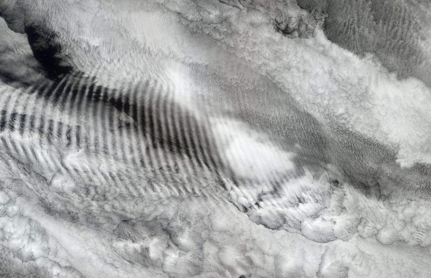
Cloud height and type also affect observing differently. A thin veil can weaken faint contrast while leaving bright planets visible; thick low cloud can block the sky entirely. The NASA reference photographs show real atmospheric structures, but they are examples rather than classifications of today's conditions at your site. Use them to understand why “cloud cover” is an incomplete description of observing quality, not to infer an unmeasured cloud type from one percentage.
Keep weather, transparency and seeing separate
A clear sky can still have poor transparency because of haze, dust or humidity. Atmospheric seeing describes image steadiness and is another separate factor. A night favorable for wide-field constellation viewing might still be disappointing for high-resolution planetary imaging. This monthly cloud dataset does not measure all those qualities for your proposed session.
For a planet, you may tolerate some lunar glare or thin haze while demanding stable seeing. For a faint nebula, sky brightness and transparency become more important. Our Saturn tracker and new Moon planner answer different parts of that decision. Combine their geometry with current conditions rather than stretching the cloud climatology into a universal observing score. The clear separation of inputs makes your final plan easier to assess.
What the NASA images contribute
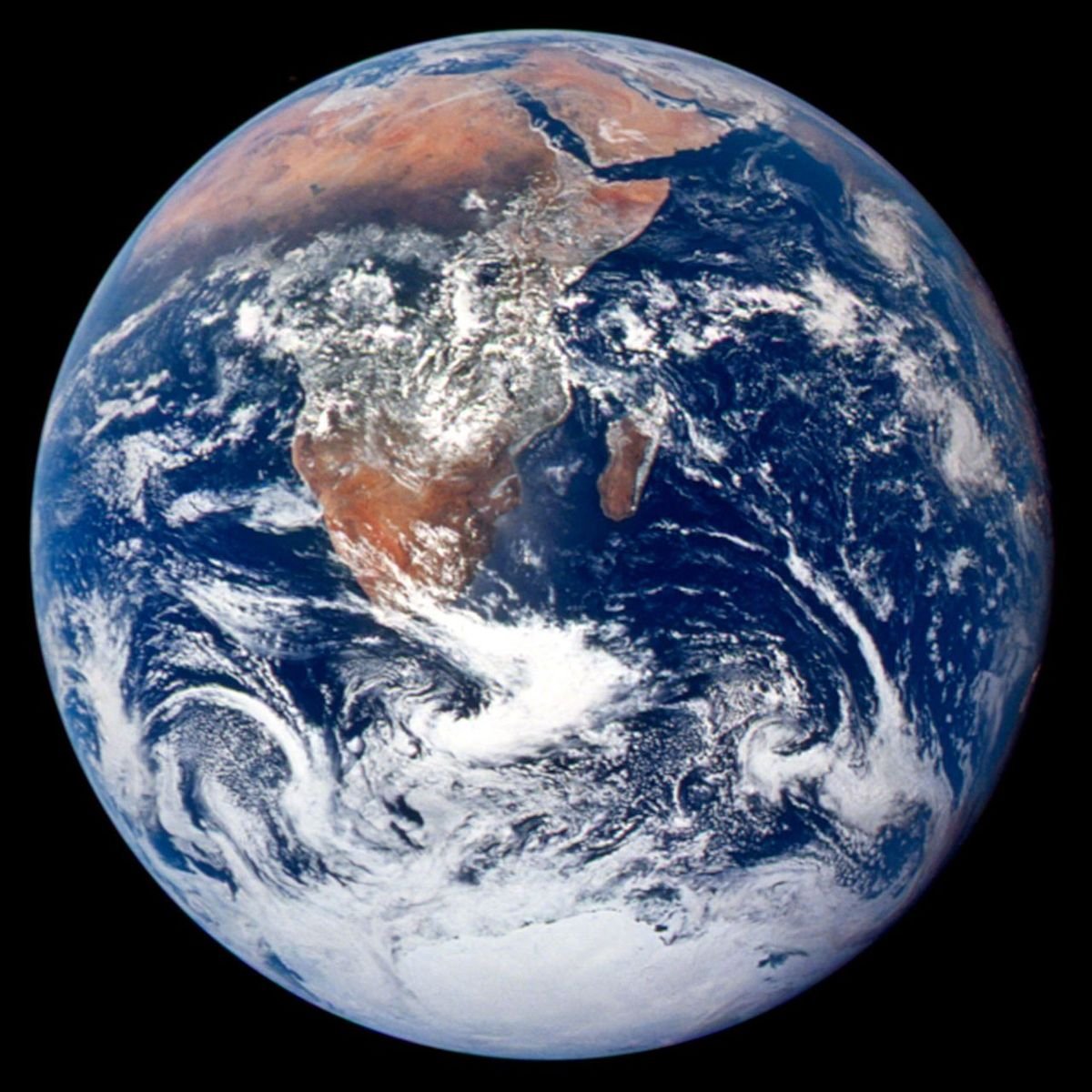
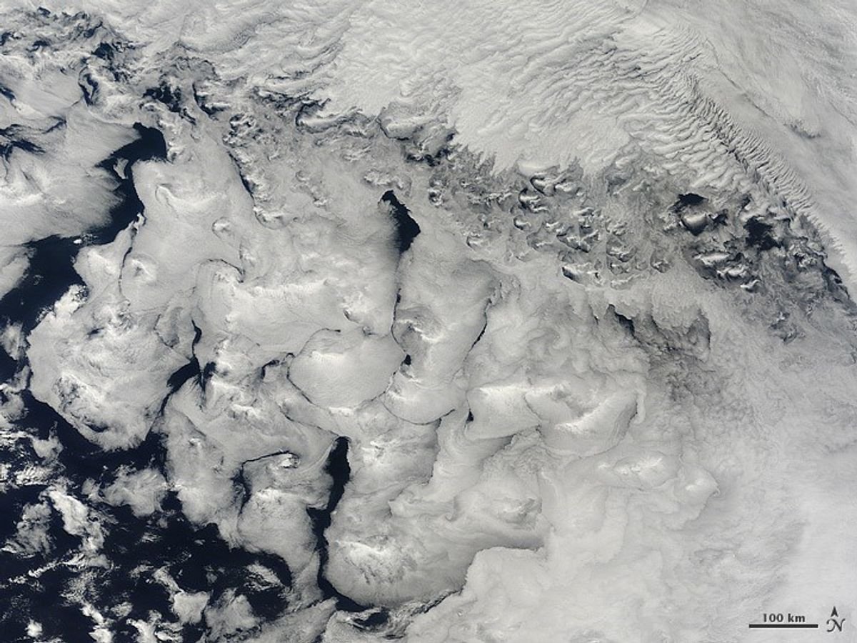
The Blue Marble picture shows Earth as a physical world with an atmosphere, while the cloud images show real patterns over ocean regions. These are NASA source images with their original credits and links. They are related to the subject of cloud structure and coverage, but they are not live views of the highlighted grid cell or photographs retrieved for your selected month.
Ocean cloud patterns can be striking and organized, illustrating that cloudiness varies in space as well as time. That does not mean the same pattern occurs around every inland observing site. Read each caption's origin and instrument context. The visual references provide scientific background; the map's numerical cells come from the NASA POWER response. Keeping image provenance and data provenance distinct prevents a historical photograph from being mistaken for the tool's current measurement.
Resolution and geographical boundaries
The cloud source is coarse, approximately degree-scale rather than neighbourhood-scale. Coastal areas, mountains and local weather regimes may vary within a single cell. A grid value close to your coordinates therefore remains a regional reference. It cannot resolve whether one hilltop or one side of a valley will have a better sky on a specific night.
Near the poles or the international date line, the requested rectangle is clipped to the service's global latitude and longitude boundaries. The tool does not wrap a second region across the date line or fill an absent cell with a guessed value. If the service cannot supply a usable regional response, an explicit error is shown. This is more useful than keeping an old map visible without warning, especially when comparing potential destinations far apart.
Turn the numbers into a sensible observing plan
Use the chart to shortlist seasons, note the dataset's historical range, and compare the target visibility for those dates. Closer to departure, check a current forecast and the local observing environment. On the night, use the actual sky as the final evidence. If clouds are intermittent, consider bright targets and short sessions rather than assuming that a monthly average rules the evening in or out.
The personalized star map can preserve the intended sky for your chosen date, giving you a clear reference when the conditions allow. Save your own outcome in an observing log too: the local experience adds context that a coarse climatology cannot provide. A careful plan uses long-term averages to choose when to try and current observations to decide what is possible.